Analysis of Data:​
Correlation:
In statistics and probability theory, correlation means how closely related two sets of data are.
Correlation does not always mean that one causes the other. It is very possible that there is a third factor involved.
Correlation usually has one of two directions.
These are positive or negative. If it is positive, then the two sets go up together. If it is negative, then one goes up while the other goes down.
Lots of different measurements of correlation are used for different situations. For example on a scatter graph, people draw a line of best fit to show the direction of the correlation .
Formula for calculating the correlation coefficient:
The formula for the correlation is:
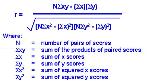
The symbol r Stand for the correlation.
Analysis of Data > Example of Correlation:

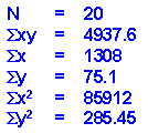
Now, when we plug these values into the formula given above, we get the following

Simple Regression:
Simple regression is used to examine the relationship between one dependent and one independent variable. After performing an analysis, the regression statistics can be used to predict the dependent variable when the independent variable is known. Regression goes beyond correlation by adding prediction capabilities.
For example, a medical researcher might want to use body weight (independent variable) to predict the most appropriate dose for a new drug (dependent variable). The purpose of running the regression is to find a formula that fits the relationship between the two variables. The regression line (known as the least squares line) is a plot of the expected value of the dependent variable for all values of the independent variable. Technically, it is the line that "minimizes the squared residuals". The regression line is the one that best fits the data on a scatter plot.
Using the regression equation, the dependent variable may be predicted from the independent variable. The slope of the regression line (b) is defined as the rise divided by the run. The y intercept (a) is the point on the y axis where the regression line would intercept the y axis. The slope and y intercept are incorporated into the regression equation. The intercept is usually called the constant, and the slope is referred to as the coefficient. Since the regression model is usually not a perfect predictor, there is also an error term in the equation.
In the regression equation, y is always the dependent variable and x is always the independent variable. Here are three equivalent ways to mathematically describe a linear regression model.
y = intercept + (slope x) + error
y = constant + (coefficient x) + error
y = a + bx + e
Calculation of regression equation:
In the table below, the xi column shows scores on the aptitude test. Similarly, the yi column shows statistics grades. The last two rows show sums and mean scores that we will use to conduct the regression analysis.
|
Student |
xi |
yi |
(xi-x) |
(yi-y) |
(xi-x)2 |
(yi-y)2 |
(xi-x)(yi-y) |
|
1 |
95 |
85 |
17 |
8 |
289 |
64 |
136 |
|
2 |
85 |
95 |
7 |
18 |
49 |
324 |
126 |
|
3 |
80 |
70 |
2 |
-7 |
4 |
49 |
-14 |
|
4 |
70 |
65 |
-8 |
-12 |
64 |
144 |
96 |
|
5 |
60 |
70 |
-18 |
-7 |
324 |
49 |
126 |
|
|
|
|
|
|
|
|
|
|
Sum |
390385 |
|
|
730 |
630 |
470 |
|
|
|
|
|
|
|
|
|
|
|
Mean |
78 77 |
|
|
|
|
|
|
The regression equation is a linear equation of the form: Å· = b0 + b1x .
To conduct a regression analysis, we need to solve for b0 and b1.
Computations are shown below.
b1 = Σ [ (xi - x)(yi - y) ] / Σ [ (xi - x)2] b1 = 470/730 = 0.644
b0 = y - b1 * x b0 = 77 - (0.644)(78) = 26.768
Therefore, the regression equation is: Å· = 26.768 + 0.644x .
Measures of Central Tendency:
Measures of Central Tendency show the tendency of data to cluster around a central value. They give us a single value that represents the whole series of data. Following are the measures of central tendency:
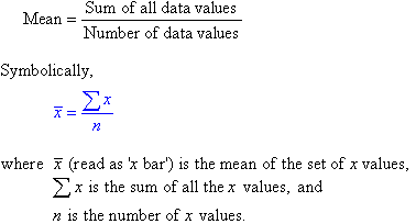
Mean:
The mean (or average) of a set of data values is the sum of all of the data values divided by the number of data values.
That is:
Analysis of Data > Example of Mean:
The marks of seven students in a mathematics test with a maximum possible mark of 20 are given below:
15 13 18 16 14 17 12
Find the mean of this set of data values.
Solution:
Mean = Sum of all the data values / Number of data values
​Mean = 15+13+18+16+14+17+12 / 7
Mean = 105 / 7
​Mean = 15
So, the mean mark is 15.
Median:
The median of a set of data values is the middle value of the data set when it has been arranged in ascending order. That is, from the smallest value to the highest value.
Analysis of Data > Example of Median:
The marks of nine students in a geography test that had a maximum possible mark of 50 are given below:
47 35 37 32 38 39 36 34 35
Find the median of this set of data values.
Solution:
Arrange the data values in order from the lowest value to the highest value:
32 34 35 35 36 37 38 39 47
The fifth data value, 36, is the middle value in this arrangement.
So median is: 36
Note:
The number of values, n, in the data set = 9
Median = 1/2(9+1)th value
Median = 5th value
Median = 36
In general:
Median = 1/2(n+1)th value, where n is the number of data values in the sample.
​If the number of values in the data set is even, then the median is the average of the two middle values. ​
Analysis of Data > Example 2 of Median:
Find the median of the following data set:
12 18 16 21 10 13 17 19
Solution:
Arrange the data values in order from the lowest value to the highest value:
10 12 13 16 17 18 19 21
The number of values in the data set is 8, which is even. So, the median is the average of the two middle values.
Median = 4th data value + 5th data value / 2
Median = 16+17 / 2
Median = 33 / 2
Median = 16.5
Note:
- Half of the values in the data set lie below the median and half lie above the median.
- The median is the most commonly quoted figure used to measure property prices. The use of the median avoids the problem of the mean property price which is affected by a few expensive properties that are not representative of the general property market.
Mode:
The mode of a set of data values is the value(s) that occurs most often.
The mode has applications in printing.
For example, it is important to print more of the most popular books; because printing different books in equal numbers would cause a shortage of some books and an oversupply of others.
Likewise, the mode has applications in manufacturing.
For example, it is important to manufacture more of the most popular shoes; because manufacturing different shoes in equal numbers would cause a shortage of some shoes and an oversupply of others.
Analysis of Data > Example of Mode:
Find the mode of the following data set:
48 44 48 45 42 49 48
Solution:
The mode is 48 since it occurs most often.
Note:
- It is possible for a set of data values to have more than one mode.
- If there are two data values that occur most frequently, we say that the set of data values is bimodal.
- If there is no data value or data values that occur most frequently, we say that the set of data values has no mode.
Requisites of a good measure of Central Tendency:
According to Prof. Yule, the following are the requirements to be satisfied by an ideal average or measure of central tendency.
- It should be rigidly defined.
- It should be easy to understand and calculate.
- It should be based on all the observations.
- It should be suitable for further mathematical treatment.
- It should be affected as little as possible by fluctuations of sampling.
- It should not be affected much by extreme observations
Measures of Dispersion:
Measures of dispersion show the variability of data from the central value. The measures of dispersion describe the width of the distribution.
Range:
The range, R, of the data is the difference of the highest and smallest values being analyzed.
Analysis of Data > Example: {1, 3, 8, 3, 7, 11, 8, 3, 9, 10}
R = 11 - 1 = 10
Deviation:
The deviation is the difference of each value from the mean. This is used in the calculation of the standard deviation and variance. "x" is the point of interest. The sum of deviations from the mean is always zero.
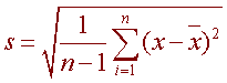
Standard Deviation:
The standard deviation is shown by the following formulas. It also equals the square root of the variance. "x" is the point of interest.
"n" represent the sample size,
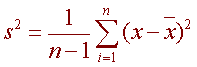
Variance:
The variance is the standard deviation squared. ​
Probability distribution:
In probability theory and statistics, a probability distribution identifies either the probability of each value of a random variable (when the variable is discrete), or the probability of the value falling within a particular interval (when the variable is continuous). The probability distribution describes the range of possible values that a random variable can attain and the probability that the value of the random variable is within any (measurable) subset of that range.
Normal distribution:
In probability theory, the normal (or Gaussian) distribution, is a continuous probability distribution that is often used as a first approximation to describe real-valued random variables that tend to cluster around a single mean value. The graph of the associated probability density function is “bell”-shaped, and is known as the Gaussian function or bell curve.
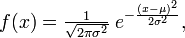
where parameter μ is the mean(location of the peak) and σ 2 is the variance (the measure of the width of the distribution). The distribution with μ = 0 and σ 2 = 1 is called the standard normal.
where parameter μ is the mean (location of the peak) and σ 2 is the variance (the measure of the width of the distribution). The distribution with μ = 0 and σ 2 = 1 is called the standard normal.
The normal distribution is considered the most “basic” continuous probability distribution due to its role in the central limit theorem, and is one of the first continuous distributions taught in elementary statistics classes. Specifically, by the central limit theorem, under certain conditions the sum of a number of random variables with finite means and variances approaches a normal distribution as the number of variables increases. For this reason, the normal distribution is commonly encountered in practice, and is used throughout statistics, natural sciences, and social sciences as a simple model for complex phenomena.
January 08, 2018